
Testing theories that go beyond the regime of applicability of Luttinger-liquid theory
We use an array of 1D wires to measure nonlinear tunnelling from the wires to a neighbouring 2D system what acts as a spectrometer for energy and momentum.
Momentum-dependent power law measured in an interacting quantum wire beyond the Luttinger limit
Power laws in physics have until now always been associated with a scale invariance originating from the absence of a length scale. Recently, an emergent invariance even in the presence of a length scale has been predicted by the newly-developed nonlinear-Luttinger-liquid theory for a one-dimensional (1D) quantum fluid at finite energy and momentum, at which the particle’s wavelength provides the length scale. We have observed experimental evidence for this new type of power law in the spectral function of interacting electrons in a quantum wire using a transport-spectroscopy technique. The momentum dependence of the power law in the high-energy region matches the theoretical predictions, supporting not only the 1D theory of interacting particles beyond the linear regime but also the existence of a new type of universality that emerges at finite energy and momentum.

Fig. 1. Overlapping 1D and 2D spectral functions.
Figure 1 above shows spectral functions, which represent with colour the available values of momentum and energy in the system of electrons, which fill all the states up to the Fermi energy EF. We put two such 2D or 1D systems one on top of the other. Using a magnetic field B (parallel to the 2D layers) we can move one in momentum relative to the other until the densest parts of their respective spectral functions overlap (a and b in the figure). We can also offset them in energy by applying a voltage VDC between the layers. If empty states in one of the systems coincide with filled states in the other, electrons can tunnel between the systems, giving a measurable current. Thus we can map out the spectral function as a function of momentum and energy using the magnetic field B and VDC, respectively. (c) shows a 2D spectral function (in blue) overlapping a 1D spectral function (in red), which has structure corresponding to the quantised subbands in the 1D system. in this way we can map out that structure, and look for evidence of electrons interacting with each other.
The theory of these charge and spin excitations is well described by Tomonaga-Luttinger-liquid theory, and we observed the two excitations travelling at different speeds ('spin-charge separation') in our maps.1 However, this theory only applies at very low excess energy (low VDC), whereas we see the spin-charge separation persisting to much higher energy. We have therefore studied the high-energy regime in great detail2-5, to look for signatures of the latest theories that go beyond the linear Luttinger regime. This nonlinear theory predicts "replicas" of the usual parabolic curves, as well as an enhanced current when probing below the "bottom" of the 1D spectrum, related to exciting multiple particles, as indicated in Fig. 2 below.

Fig. 2. (a) Dispersion (energy E vs momentum ℏk) of an interacting 1D system. White is the kinematically forbidden region and grey is the continuum of many-body excitations. The thick red line separates the border between the two regions. The states on the border that form it correspond to removing a single particle (marked by a black circle at k1) from the many-particle state, and an excitation described by the mobile-impurity model marked by a green circle. (b) Splitting of the fermionic dispersion into two subbands, one for the heavy hole with velocity ~k1/m and one for the excitations around EF with velocity vF. The green circles are the constituent parts of the many-body excitations in the nonlinear regime.
The devices used to measure the dispersion relation (energy E vs momentum ℏk) of an interacting 1D system consisted of a GaAs/AlGaAs heterostructure with two parallel quantum wells 100nm beneath the surface, both 18nm wide, separated by a 14nm tunnel barrier. Fig. 3 is an illustration of the device structure. An array of identical 1D channels is defined in the uppoer well using metal gates on the surface. A current of electrons is injected into these wires and the electrons tunnel through the barrier into the 2D well below. As energy and momentum (related to the electrons' quantum-mechanical wavelength) are conserved, tunnelling depends on the energy and momentum of electrons and empty states in the two layers, so we can map out the electron dispersion relation in the 1D channels by varying the voltage VDC between the layers (to change the energy) and the magnetic field B in the plane of the layers (to change the momentum). In Fig. 4(a), the conductance G = I/VDC is plotted, showing parabolae that correspond to the dispersions of the 1D and 2D systems.
| (a) |  |
| (b) |  |
| (c) |  |
Fig. 3. (a) Illustration of the 1D-2D spectrometer device. The control gates are split gate (SG) and mid-gate (MG) (depleting the lower layer but not the top, to inject current into the upper layer), gates defining 1D wires (WG), gate over the parasitic region (PG), and barrier gate (BG) confining the upper layer. Gates are not drawn to scale. In reality they consist of a three-column array of over 500 wires, each of length 18μm and gate width 0.1μm, with 0.18μm separation (device A) and 10μm and gate width 0.3μm, with 0.2μm separation (device B).
(b) Schematic of current flow: current enters top layer under mid-gate MG at left, flows into 1D wires (blue) via parasitic regions (magenta, labelled P), and tunnels to lower, 2D, layer and out to a contact at the right.
(c) Scanning electron micrograph of a device, showing the air bridges. The scale bar is 5μm long.
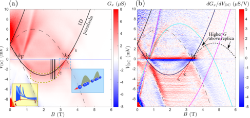
Fig. 4. a) Overview of conductance G against B (∝ momentum) and voltage VDC (∝ energy eVDC) (Sample A). The region along which G is enhanced is shown enclosed by a dashed yellow line, and the left inset shows how G might decay with energy, differently for each momentum k. Vertical black lines show cuts along which fitting is carried out. The region where spin-charge separation is visible is shown enclosed by a dashed blue line; the right inset illustrates charge (dots) and spin (shaded) waves. The bottom edge of the yellow region is selected as the line above which the nonlinear-Luttinger-liquid model still gives a reasonable fit.(b) Differential dG/dVDC of the raw data in (a), showing a replica above the Fermi wavevector kF (where the conductance stays higher than expected for the non-interacting model in the region labelled Higher G, and then appears to drop off along a parabola that is an inverted replica of the main 1D parabola), separate spin and charge lines near VDC = 0, labelled S and C, respectively, and the parasitic signal (near magenta and cyan lines).
The figure below shows cuts through the spectrum of the conductance G measured as a function of VDC at various magnetic fields. The continous curves are measured data, and the dots are the values calculated using the latest theory. Crosses are the conductance calculated using a model assuming no interactions. Note the enhancement of G at the left of Fig. 5(a) above the crosses, matching the new theory, which includes a momentum-dependent power-law behaviour of the tunnelling.

Fig. 5. Fitting results showing the interaction-induced enhancement to the left of the peak. Fits to the conductance for (a) sample A and (b) sample B, normalised to their peak values and shifted vertically for clarity, for a model without interactions (crosses) and the model with interactions (dots). The dashed lines show the confidence interval of the measurement data within estimated error of the background conductance subtraction. The broadening fitting parameters for the non-interacting and interacting models (ΓNI and ΓI, respectively) are shown, in units of meV, together the magnetic field B at which the data were taken. Sample A (wires 18μm long) was measured at 50mK in a 3He/4He$ dilution refrigerator, while sample B (10μm long) was measured at 330mK in a 3He cryostat.
(c) Fits using other theories, or matching different parts of the data using different constant exponents α1 and α2, as labelled (using data for sample A).
In summary, we have studied experimentally the decay of the tunnelling current below the bottom of the 1D subband. The conductance G decays more slowly than predicted by the non-interacting theory, or by interacting theory that includes only a fixed power law. A good fit, however, is obtained using a power law that depends on momentum, as predicted by the recent theory. This appears to be the first example of an interaction-driven variable power law.
References
1“Probing Spin-Charge Separation in a Tomonaga-Luttinger Liquid”, Y. Jompol, C. J. B. Ford, J. P. Griffiths, I. Farrer, G. A. C. Jones, D. Anderson, D. A. Ritchie, T. W. Silk and A. J. Schofield, Science, 325, 597–601 (2009).
2“Hierarchy of Modes in an Interacting One-Dimensional System”, O. Tsyplyatyev, A. J. Schofield, Y. Jin, M. Moreno, W. K. Tan, C. J. B. Ford, J. P. Griffiths, I. Farrer, G. A. C. Jones and D. A. Ritchie, Phys. Rev. Lett., 114, 196401 (2015).
3“Nature of the many-body excitations in a quantum wire: Theory and experiment”, O. Tsyplyatyev, A. J. Schofield, Y. Jin, M. Moreno, W. K. Tan, A. S. Anirban, C. J. B. Ford, J. P. Griffiths, I. Farrer, G. A. C. Jones and D. A. Ritchie, Phys. Rev. B, 93, 075147 (2016).
4“Nonlinear spectra of spinons and holons in short GaAs quantum wires”, M. Moreno, C. J. B. Ford, Y. Jin, J. P. Griffiths, I. Farrer, G. A. C. Jones, D. A. Ritchie, O. Tsyplyatyev and A. J. Schofield, Nat. Commun., 7, 12784 (2016).
5“Momentum-dependent power law measured in an interacting quantum wire beyond the Luttinger limit”, Y. Jin, O. Tsyplyatyev, M. Moreno, A. Anthore, W. K. Tan, J. P. Griffiths, I. Farrer, D. A. Ritchie, L. I. Glazman, A. J. Schofield and C. J. B. Ford, Nat. Commun., 10, 2821 (2019).